p_heads <- 60/(60+40)
p_heads
[1] 0.6We start our first look at GLMs with binary regression. Here, we consider when binary regression, specifically logistic regression, is more appropriate than a regular (general linear) regression. We will also fit toy data and interpret the results.
When the outcome is a binary variable, or when there are only two possible outcomes, there are two essential problems with using the general linear model (e.g., the regular lm() function) . The first essential problem is due to the non-normal shape of the residuals. The second essential problem is that the outcome variable is not continuous and normally distributed. Both problems contribute to general linear models being biased and making impossible predictions.
Binary regression is a general term that encompasses specific models such as logistic regression and probit regression. It is a way to analyze binary data and hold the assumptions of linear models more true. We will focus on logistic regression in this module.
Terms
Binary Regression: A general term for models for when the outcome variable has only two possible outcomes.
Logistic Regression: A specific binary regression model which uses the logistic function as the link function.
Probit Regression: A specific binary regression model which uses the probit function as the link function.
Link Function: A function that transforms the outcome variable into a continuous and unbounded variable. It is a key aspect of generalized linear models.
The general linear model assumes that residuals, or the differences between the observed and predicted values of data, are normally distributed. If the residuals are not normally distributed, the model is likely to make invalid inferences or predictions.
Since the outcome variable is binary, a quick histogram plot will show that it is not continuous (i.e., it is discrete). This is a scourge for the general linear model since it assumes continuous and normally distributed outcomes, and it will predict both intermediate states/values between the two possible outcomes and states/values above and below the two possible outcomes.
For example, if 0 = Alive, and 1 = Dead, then the general linear model may predict a value between 0 and 1 (somewhere between alive and dead), or values below 0 and above 1 (so less alive and more dead?).Therefore, to model a binary outcome using the machinery of linear modeling, we need to transform the outcome variable to a continuous and normally distributed outcome.
As mentioned earlier, in logistic regression we are modeling a binary events. When we can assume that 1) Binary events are independent of one another (i.e., one binary trial doesn’t affect another trial), and 2) The probability of the binary event happening versus not happening is fixed, then it turns out that binary events are best described by what’s called a binomial distribution. In theory, it is the optimal distribution for a binary event based on a principle called Maximum Entropy, but we will skip that theoretical explanation for now.
A binomial distribution is described by only two parameters: n and p. The “n” parameter is the total number of trials/events, and “p” is the probability of a “success” (or the probability of the event happening versus not happening). Due to this feature of binomial distribution, we can expect the mean of a binary event to simply be the number of trials multiplied by the probability of the event occurring, or \(n * p\). For example, if we flip a coin 100 times and count the number of Heads, we can expect the average number of Heads after 100 flips to be \(n*p = 100 * 0.5 = 50\, Heads\).
The important thing to know is that logistic regression’s goal is to model the “p” parameter, or the probability of success, of a binary distribution with a linear and additive combination of an intercept and slope of a predictor variable(s). But there’s an inherent problem with modeling probability with a linear model because probability is bounded from [0,1], and we already know that a linear model works best when the outcome is unbounded (and continuous).
At this point, we need to make a distinction between the outcome of a binary event and the probability of a binary event. Because logistic regression’s goal is to model the probability of a binary event rather than the outcome of a binary event.
The outcome of a binary event is the result of the trial – whether the event was a success or not. The way we define which one of two outcomes of a binary event is a “success” is arbitrary and depends on our goals. For example, if 0 = Dead, and 1 = Alive, the “success” or outcome we are concerned with is being alive.
The probability of a binary event is not the result of the trial. It is the model’s estimation of the chance or likelihood of the “success” of the trial, i.e., the probability of one of the two events occurring. As a review, if the probability of one event = p, then 1-p is the probability of the other event.
As mentioned in the previous section, the logistic regression model takes into account that the outcome we are modeling is a binary outcome, and its goal is to model the probability of a binary event (since this is the parameter of the binomial distribution we are concerned with). Since a probability is a value that is bounded between [0,1], we need a way to modify the linear model to work with probability. We are motivated to do this because the linear model works best when the outcome it is modeling is a unbounded (and continuous), but probability is clearly bounded between [0,1].
Let’s summarize the details of this model in a more compact way:
\[ y_i \sim Binomial(n,p)\] Here we are saying that our outcome variable is binomially distributed. This is not the part of the model that logistic regression is specifically concerned with – this is an assumption we are placing on the model knowing that the data is a binary outcome.
\[ g(p) = \beta_0 + \beta_1 x_1\] Here we are now defining how we use the simple logistic regression model. We call it simple because there is only one predictor variable (\(x_1\)). The right side of the equation should be very familiar to us: it is a linear model where we have \(\beta_0\) (the intercept), and \(\beta_1\) (the slope of the predictor variable).
But the left side of this equation is unique to generalized linear models. First, we see that we are assigning \(\beta_0\) and \(\beta_1\) to estimate \(p\), which is the probability parameter of the binomial distribution. However, we also see that \(p\) is inside a function called \(g\), which we now define as our link function.
The link function will allow us to use the linear model (the right side of the equation that is usually assumed with a continuous and unbounded outcome) to estimate probability, \(p\), which is continuous and bounded.
In logistic regression, our \(g\) is the “logit function”, which is defined as:
\[ g = log(p/(1-p)) \] or, equivalently,
\[ p = e^g/ (1 + e^g) \]
When we use the logit link function with a linear predictor, we now can call this “logistic regression”.
When we use GLMs, we will be using many different link functions depending on the data. In the case of binary/logistic regression, all this function is trying to do is relate our linear predictors to a response outcome that is continuous and between some bounds (like 0 and 1). More generally, we need link functions because if we did not do this, we are using the linear predictors to predictor some value that is continuous when it may not continuous (like discrete values for binary variables), and the predictions can be out of bounds (like when an event “yes” = 1, then the model can spit out a value like 1.53, even though this event is unreasonable). We also find that when using the appropriate link function, other problems, like the shape of residuals, gets fixed!
Before we fit our first logistic regression, let’s take a look at what is actually happening and why the generalized linear model is similar, but different, to the general linear model.
In simple regression, we are predicting the outcome (\(y_{{i}}\)) with a linear (additive) combination of an intercept (\(\beta_0\)) and one predictor variable (\(x\)).
\[ \hat{y}_{{i}} = \beta_0 + \beta_1 x \] In simple logistic regression, we are still predicting an outcome with a linear (additive) combination of intercept and one predictor variable. We use the term “simple” only because we have one predictor variable in this case.
\[ \hat{g}_{i} = \beta_0 + \beta_1 x \]
Note that the linearly additive feature that both simple linear regression and simple logistic regression share is what makes these models related and interpretable.
The main difference is why, in simple logistic regression, did the outcome variable change from \(y_{{i}}\) to \(g_{i}\)? Because in binary regression, we are no longer predicting the binary outcome event (e.g., “yes/no”). Usually (but not always) we are predicting the probability of the binary event occurring. This means that \(\eta_{i}\) is a probability that is bounded between 0 (“no” event) and 1 (“yes” event).
Now, we will relate \(y_{\hat{i}}\) to \(g_{i}\).
We need to make a connection between the probability of an event (\(g_{i}\)) to an event outcome (\(y_{{i}}\)). This is possible in this way:
The outcome \(y_{{i}}\) for i = 1,…,\(n\) events takes values zero or one with the probability of a 1 = \(p_i\)
In other words, \(P(Y_i = 1)\) = \(p_i\), or P is the probability of a 1 (e.g., “yes” happening).
That is all just setup to define \(g_{i}\).
The variable \(g\) is our “link function”. In this case, it is a function that transforms a probability (\(p_i\)) into our \(\eta_{i}\). Therefore, we are trying to find the probability of an event occurring.
When working with logistic regression, we have to be familiar with the model’s units, or frame of reference for its parameter estimates. When logistic regression models estimated, they are usually presented in log-odds, but, as we will see now, it is fairly straightforward to transform our units from log-odds to odds to probability.
Note that we are doing these calculations here by hand solely as an exercise to familiarize ourselves with these units. This is not actually required when running logistic regressions. Indeed, like with lm(), we will be given results tables which calculate all of these for us.
As an example, imagine flipping a coin 100 times. As an arbitrary decision, let’s consider the results of this binary event that when a coin lands on Heads, it is a Success. And when it lands on Tails, it is a failure. In this example, it lands Heads 60 times out of 100.
Probability The probability of landing a head is:
p_heads <- 60/(60+40)
p_heads[1] 0.6Notice that the probability is a proportion/ratio of Heads out of the total number of coin flips.
Odds
o_heads <- p_heads/(1 - p_heads)
o_heads
[1] 1.5Odds is simply another way of describing probability. It is also a ratio, like probability, but essentially with odds you can have some way to describe the relative likelihood of the event occurring versus not occurring. For example, if the probability of an event occurring is 0.75 or 75% likely, its odds of happening is “3 to 1”, or it is 3 times more likely that the event will occur relative to it not occurring.
0.75/(1-0.75)[1] 3In the case of the data, the odds for flipping a Heads is 1.50.
Working with odds can be challenging at first but there is a rule of thumb to follow. Imagine if \(p=.50\), then it is 50% chance of an event occurring or not occurring. Then, when we convert this to odds, then \(odds= .50/.50 =1\). So, if you get an odds value that equals 1 , then both events are equally likely, and if it less than 1, then it is less likely for an event to occur, and if it is more than one, it is more likely for an event to occur.
It seems like flipping Heads 60 times out of 100 is more likely with a value of 1.50
Log-Odds
log_heads <- log(o_heads)
log_heads
[1] 0.4054651You might wonder why we make an effort to convert odds to log-odds. Well, again, it is because it our logistic link function that takes our outcome variable and transforms it into a continuous and bounded outcome variable so that it can work well with linearly additive predictors variables.
Just like with odds, there we can consider a rule of thumb where if \(odds=1\) then the $log odds=ln(1)=0 $. So, if we obtain a log-odds value of 0, then the event is equally likely to occur or not occur.
Our data shows a log-odds of \(0.41\), which means it is more than 0, so we can see that it is more likely (in terms of log-odds) for someone to flip a Head than a Tail.
The data for this chapter consists of some records of passengers on the Titanic. The question we will ask and answer with binary regression is if the amount of fare contributed in some way to the survival of passengers. Since survived is a binary outcome (yes or no), this relationship is best assessed with binary regression.
In addition to our usual packages (tidyverse, easystats, and ggeffects), we will also need to load DHARMa and qqplotr in order to make our plots for our binary regression models.
# A tibble: 887 × 5
   sex      age class  fare survived
   <chr>  <dbl> <chr> <dbl> <chr>
 1 male      22 3rd    7.25 no
 2 female    38 1st   71.3  yes
 3 female    26 3rd    7.92 yes
 4 female    35 1st   53.1  yes
 5 male      35 3rd    8.05 no
 6 male      27 3rd    8.46 no
 7 male      54 1st   51.9  no
 8 male       2 3rd   21.1  no
 9 female    27 3rd   11.1  yes
10 female    14 2nd   30.1  yes
# ℹ 877 more rows
This data shows records for 877 passengers on the Titanic.
Here’s a table of our variables in this dataset:
| Variable | Description | Values | Measurement |
|---|---|---|---|
sex |
Male or Female | Characters | Nominal |
age |
Age of Passenger | Double | Scale |
class |
Category of Passenger Accommodation | Characters | Nominal |
fare |
Cost of fare | Double | Scale |
survived |
“Yes” or “No” if survived | Characters | Nominal |
In order to use the survived variable in our analyses, we need to re-code the outcomes as integer numbers. Here, we will use the mutate() function from the dplyr package (which is a package that automatically loaded with tidyverse) to add a new column to our data which re-codes “Yes” = 1 and “No” = 0.
Note that our choice of “Yes” = 1 and “No” = 0 is completely arbitrary. We could have just easily switched the coding scheme. However, it is important to understand that when “Yes” = 1 and “No” = 0, our model is predicting the likelihood of survival, and if it was the other way around (when Yes = 0 and No = 1), our model would be predicting the likelihood of not-surviving.
## Prepare the data for analysis
titanic2 <-
  titanic_data |>
  mutate(
    survived_b = case_match(
      survived,
      "no" ~ 0,
      "yes" ~ 1
    )
  )
Warning: There was 1 warning in `mutate()`.
ℹ In argument: `survived_b = case_match(survived, "no" ~ 0, "yes" ~ 1)`.
Caused by warning:
! `case_match()` was deprecated in dplyr 1.2.0.
ℹ Please use `recode_values()` instead.titanic2 #print# A tibble: 887 × 6
sex age class fare survived survived_b
<chr> <dbl> <chr> <dbl> <chr> <dbl>
1 male 22 3rd 7.25 no 0
2 female 38 1st 71.3 yes 1
3 female 26 3rd 7.92 yes 1
4 female 35 1st 53.1 yes 1
5 male 35 3rd 8.05 no 0
6 male 27 3rd 8.46 no 0
7 male 54 1st 51.9 no 0
8 male 2 3rd 21.1 no 0
9 female 27 3rd 11.1 yes 1
10 female 14 2nd 30.1 yes 1
# ℹ 877 more rowsRe-coding these strings/characters into discrete numbers is important for the model’s mathematics to work.
In addition, we will turn sex into a factor with the reference group as being females.
mutate() is a function from dplyr that adds a column to the dataframe (the object that holds the data). This isn’t the only way to accomplish our goal of re-coding survived, but it is a fairly elegant, easy, and straightforward way to do so. The trick is to remember that mutate() adds a column to the existing dataframe with the same number of rows as the existing dataframe.
Our choice of data-wrangling functions are open to reprisal because there are many ways in data analysis and programming to do the same thing.
Like always, it is important to plot the data prior to fitting any model. Here, we consider if there is some sort of bivariate relationship between survived_b and fare, and survived_b and sex.
Here, we first try a scatter plots to assess a relationship between surived_b and fare. Since there are only two outcome values though, it’s hard to see any clear effect of survival based on fare.
ggplot(titanic2, aes(x = fare, y = survived_b)) +
  geom_point() + mytheme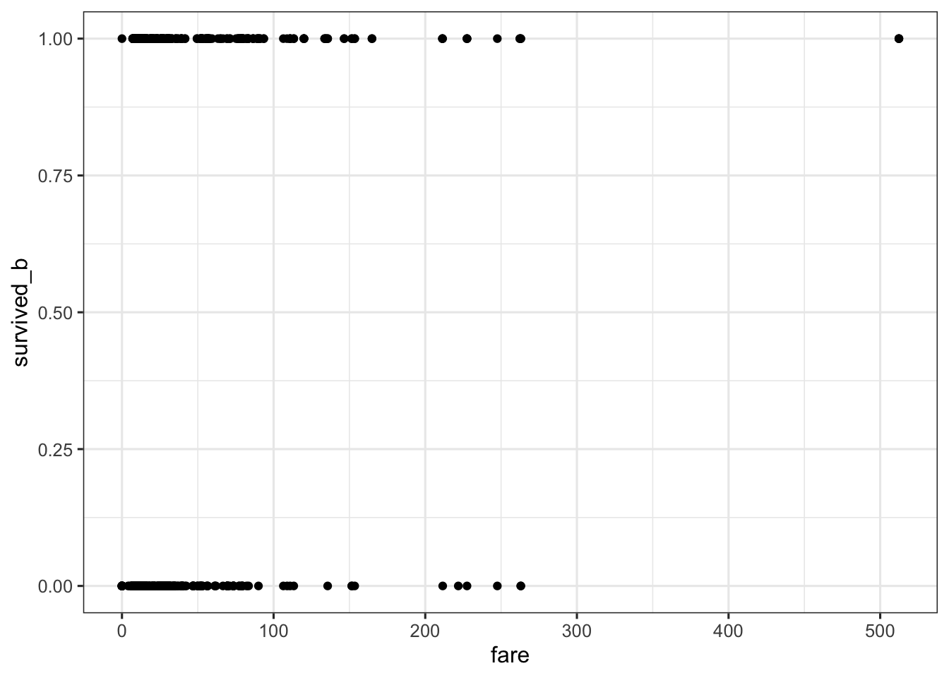
Next, we try a box plot using the original survived variable (so it is discrete again). The box plot helps clarify what the scatter plot can’t easily show: there seems to be some effect of fare on survival, such that the higher the fare, the more mass/points are in having survived the titanic. We will explore this relationship in our regression models.
ggplot(titanic2, aes(x = fare, y = survived)) +
  geom_boxplot() + mytheme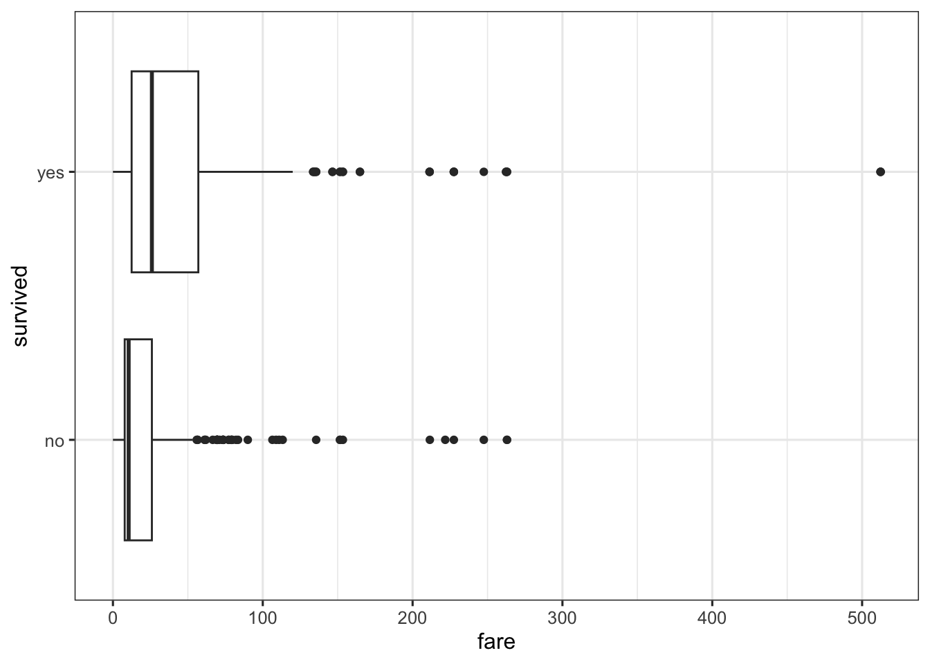
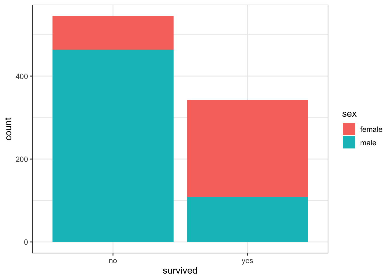
Now, let’s do a barplot for sex and survived. It seems that there is an effect on survival due to sex such that females were more likely to survive than males.
First, let’s take a look at the case for models with one dummy coded categorical predictor variable and one continuous predictor without any interaction term.
Before we fit the binary regression, it would be worthwhile to try fitting the less appropriate regular general linear model. We’ll use our old friend lm() to assess the relationship between the outcome variable survived_b with the predictor variables fare and sex. For more information on general linear modeling, we covered these topics in our Regression Recap chapter.
| Parameter | Coefficient | SE | 95% CI | t(884) | p |
|---|---|---|---|---|---|
| (Intercept) | 0.67 | 0.03 | (0.62, 0.72) | 26.01 | < .001 |
| sex (male) | -0.52 | 0.03 | (-0.58, -0.47) | -18.17 | < .001 |
| fare | 1.60e-03 | 2.76e-04 | (1.06e-03, 2.14e-03) | 5.79 | < .001 |
As the results show, we have a significant partial effect of fare, such that a 1 unit increase in fare increases the chance of survival by a small amount (0.00251 units of “survival”) while controlling for sex. In addition, we see significant effects of our dummy coded sex variable both as the intercept difference from 0 being significant (i.e., the reference group being females with an average survival of 0.67 units), and a significant difference between males and females (i.e, a decrease of 0.52 survival units for males). Despite the challenge of interpreting what units of survival are, it is worth nothing that the regular lm() “worked” in that it was able to produce an estimate.
However, it doesn’t mean that the model is the best model to use and this is evident when we plot the predictions using the predict_response() function for fare.
predict_response(fitlm1, terms = "fare") |> plot(show_data = TRUE)Data points may overlap. Use the `jitter` argument to add some amount of
random variation to the location of data points and avoid overplotting.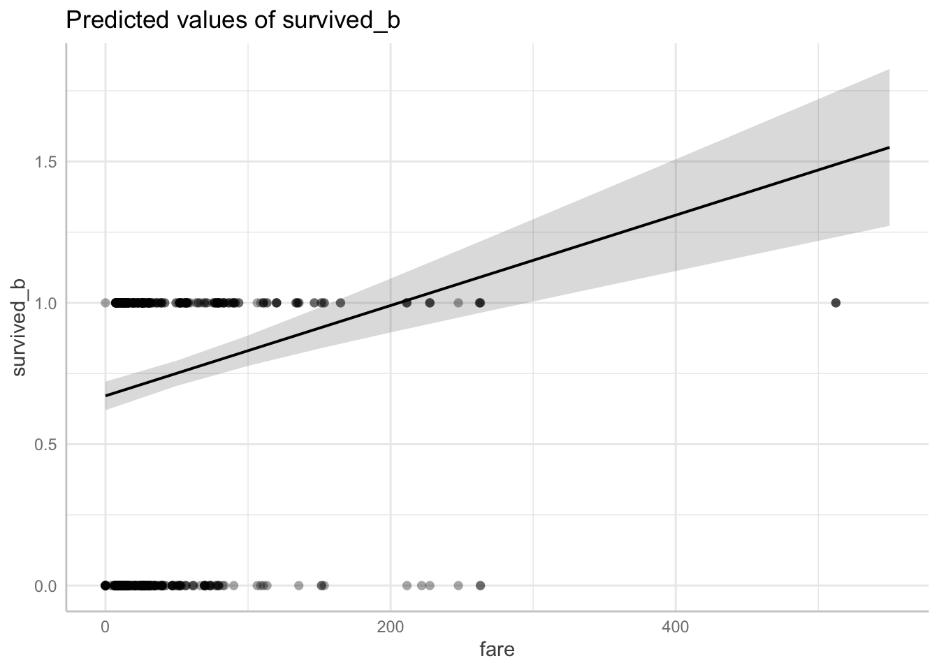
Notice that although the data points are only either 0 or 1 (binary), the regression line takes intermediate values between 0 and 1, and extreme values above 1! For example, if a passenger paid $100, then the outcome value would be ~0.25, which is somewhere between alive and dead! We can’t have passengers somewhat between alive/dead, or more or less alive/dead!
When we fit a model, we always want to see if there were any violations in the assumptions. When using the general linear model via the lm() function for binary responses, taking a look at a plot of the residuals, using check_residuals() 1, should be concerning.
## Check residuals
check_residuals(fitlm1) |> plot() # looks bad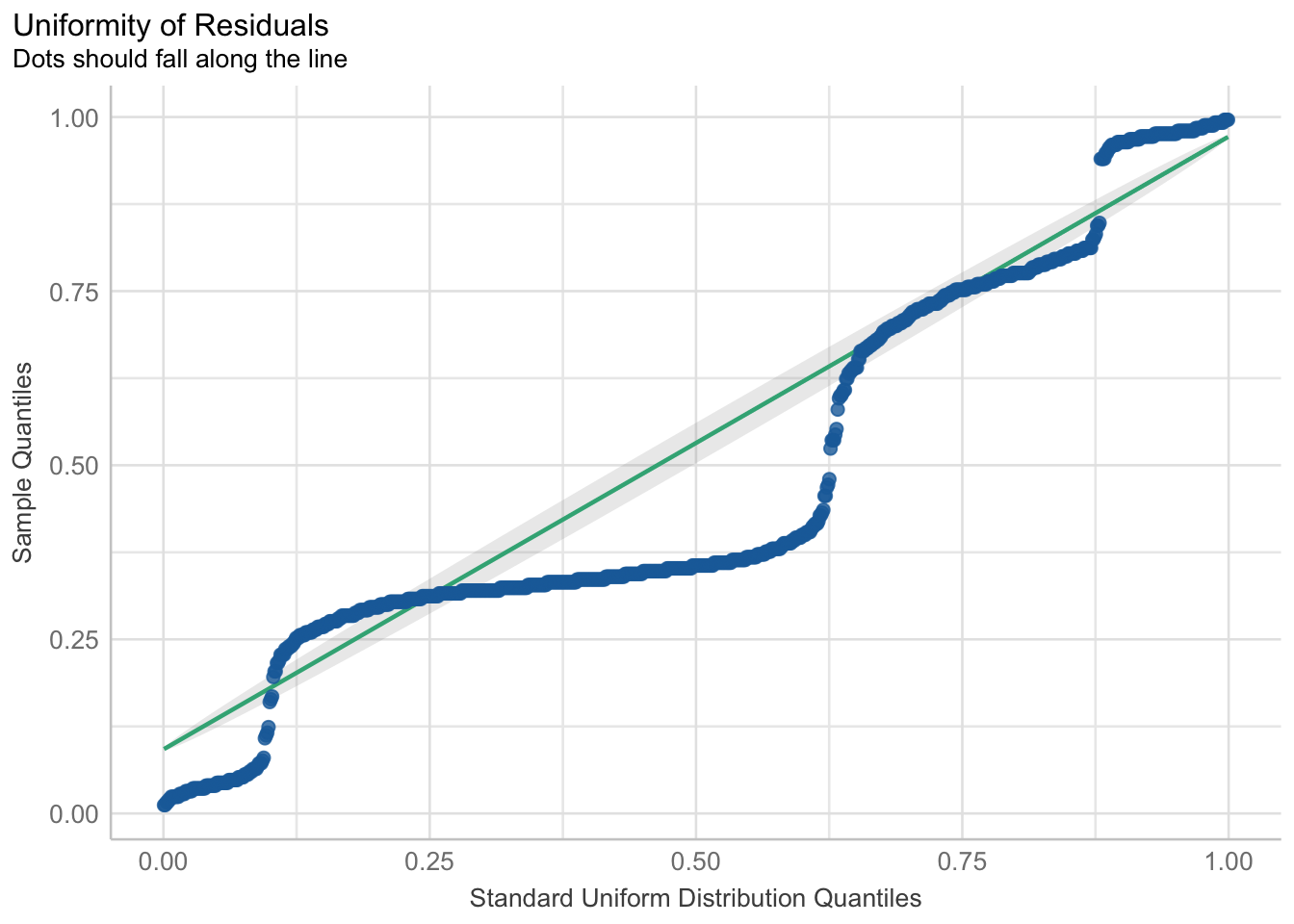
Yikes! As you can see, the dots do not fall along the line. Once this or any other assumption of the general linear model are not met, this is a clear sign that parts of the model may not be trustworthy. Specifically, in this case of the non-uniformity of residuals, there is terrible violation to the model’s uncertainty estimates; therefore, while the predictions may be okay, we can (and should) do better.
So now, finally, we fit our first GLM.
Now let’s compare our modeling of the same variables using binary/logistic regression on the interpretation of estimates and adherence to model assumptions.
“Is there a relationship between the amount of fare, sex, and the log-odds of survival?”
Again, because we have multiple predictors, multiple regression allows us to control for the effects of multiple predictors on the outcome, and we are left with the unique effect of a predictor when controlling for other predictors. In this case, the outcome variable will be survived_b, and the predictor variables will be sex (categorical variable) and fare (continuous variable).
We did a lot of work already with the lm() in the “Regression Recap”. The glm() function is in many ways the same as the lm() function. Even the syntax for how we write the equation is the same. In addition, we can use the same model_parameters() function to get our table of parameter estimates. Indeed, we will use the glm() function for the remainder of the rest of the online modules.
But notice that the glm() function has one more input argument. This input argument is the “family” input argument, which requires which “family of distributions” to use and which “link function” choice. For binary regression, we supply the binomial distribution and the logit link function.
| Parameter | Log-Odds | SE | 95% CI | z | p |
|---|---|---|---|---|---|
| (Intercept) | 0.65 | 0.15 | (0.36, 0.94) | 4.37 | < .001 |
| sex (male) | -2.42 | 0.17 | (-2.75, -2.09) | -14.16 | < .001 |
| fare | 0.01 | 2.29e-03 | (6.91e-03, 0.02) | 4.87 | < .001 |
Again, the parameter table output from a model fit with glm() looks very similar to parameter table outputs from models fit with lm(). But there is a big difference – in glm() models, we are no longer working in the same raw units!
This difference is apparent in the second column of the output table: “Log-Odds”. Because we fit a logistic regression with a logit function, the parameter values are in “log-odds” unit.
Due to the nature of the dummy coded categorical variable sex, we will assess the parameters from each level of that variable first.
The intercept is the average log-odds of surviving for female passengers while accounting for the effect of
fare. In this case, female passengers who paid no fare have an average log odds of 0.65 indiciating that female passengers are more likely to survive than not survive.
Male passengers have a 2.42 decrease in the log-odds of suriving relative to the female passengers while accounting for the effect of
fare(i.e., they have a worse chance of surviving).
Because the intercept was significant, there was a significant difference between the estimate of female passengers and 0, \(p<0.001\). Because “sex[male]” was significant, the difference between female and male passengers was significant, \(p<0.001\).
Lastly, while controlling for the effect of
sex, a one unit increase infarewas significantly related to a 0.01 increase in the log-odds of survival.
We now turn our attention to the continuous variable fare. If log-odds of fare is $ = 0.01$, then it is the case that we can say it is more likely for someone to survive the Titanic with an increase in fare paid.
This effect (fare) is also statistically significant from 0 (\(p<0.001\)).
We can easily convert log-odds to odds. In order to convert from a log-odds to odds, we just need to take the exponentiate the parameter value.
Fortunately, we can actually transform the entire log-odds parameter table results into odds using the same model_parameters() function with the added input argument of “exponentiate”, like so:
model_parameters(fit1, exponentiate = TRUE) |> print_md()| Parameter | Odds Ratio | SE | 95% CI | z | p |
|---|---|---|---|---|---|
| (Intercept) | 1.91 | 0.28 | (1.43, 2.57) | 4.37 | < .001 |
| sex (male) | 0.09 | 0.02 | (0.06, 0.12) | -14.16 | < .001 |
| fare | 1.01 | 2.32e-03 | (1.01, 1.02) | 4.87 | < .001 |
Due to the nature of the dummy coded categorical variable sex, we will assess the parameters from each level of that variable first.
The intercept is the average odds of surviving for female passengers category while accounting for the effect of
fare. In this case, female passengers have a average odd ratio of 1.91 indiciating that female passengers are more likely to survive.
Male passengers have a 0.91, or 91% decrease, in the odds of suriving relative female passenger while accounting for the effect of
fare(i.e., they have a worse chance of surviving). It is a decrease because we are talking in odds and the value is less than 1. And we interpret that value as 0.91 because 1 - 0.09 = 0.91.
There was a significant difference between the estimate of female passengers and 1, \(p<0.001\). The difference between the odds of female and male passengers was also significant, \(p<0.001\).
Lastly, while accounting for the effect of
sex, a one unit increase infarewas significantly related to a 0.01 increase, or 1% increase, in the odds of survival. It is an increase because we are talking in odds and the value is more than 1. And we interpret that value as 0.01 because 1 - 1.01 = 0.01.
A convenient transformation is taking the log-odds and converting into probability. Then, our question becomes “Is there a relationship between the sex, fare, and the probability of survival?”.
We can assess this relationship with the predict_response() function. It outputs a plot with the Y-axis as “the probability of survival_b” and the X-axis as the predictor (in this case fare) in raw units.
With predicted probabilities, while accounting for sex, we can see the probability of surviving is increasing with fare amount.
predict_response(fit1, terms = "fare") |> plot(show_data = TRUE)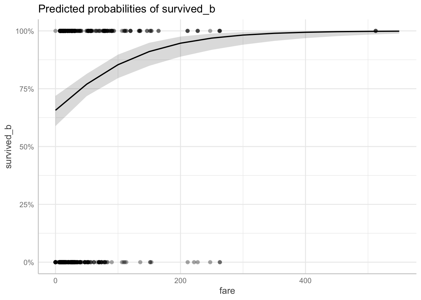
We can also plot the predicted probabilities of sex while accounting for the effect of fare.
predict_response(fit1, terms = "sex") |> plot(show_data = TRUE)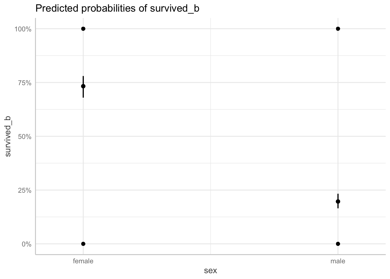
When the predicted probabilities are plotted, we can visualize the differences in probabilities of surviving between sexes.
Additionally, we can see the exact probability value for each class with the estimate_means() function.
| sex | Probability | 95% CI |
|---|---|---|
| female | 0.73 | (0.68, 0.78) |
| male | 0.20 | (0.17, 0.23) |
Variable predicted: survived_b; Predictors modulated: sex; Predictors averaged: fare (32); Predictions are on the response-scale.
Although working with probabilities seems to be more easily understandable, we cannot have parameter estimates in probabilities. Therefore, results are often communicated in logits or odds since we can have estimates, uncertainty values (like standard deviations), and significance tests applied to them.
When we use logistic regression over regular linear regression, we benefit in terms of adhering to the assumptions of the linear model. First, let’s see if our residuals are better when we used the GLM.
As we can see, compared to our residuals plot using lm(), our glm() logistic model conforms to the uniformity of residuals assumptions way better.
## Check residuals
check_residuals(fit1) |> plot() # looks way better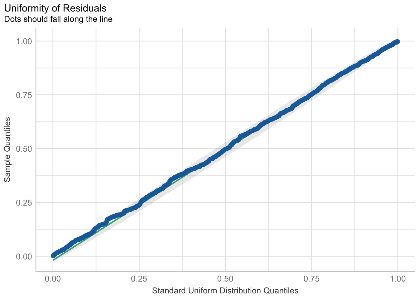
Overall, we can see the benefit of the glm() against the lm() when we compare between the two models that have the same outcome and predictors.
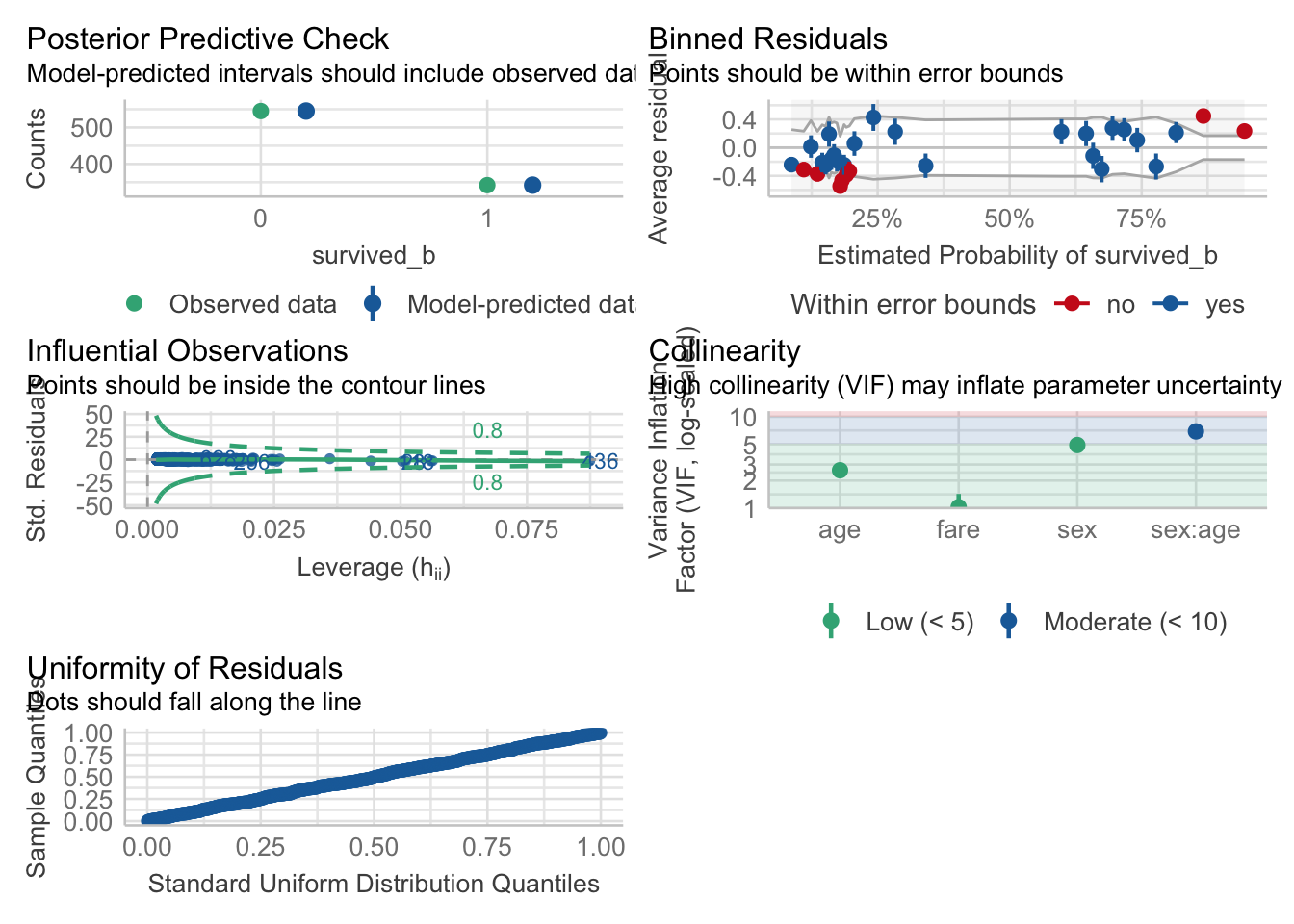
check_model(fitlm1)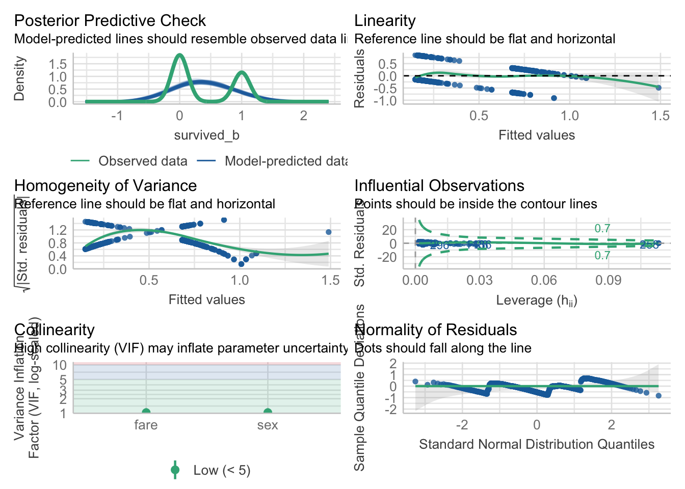
check_model(fit1)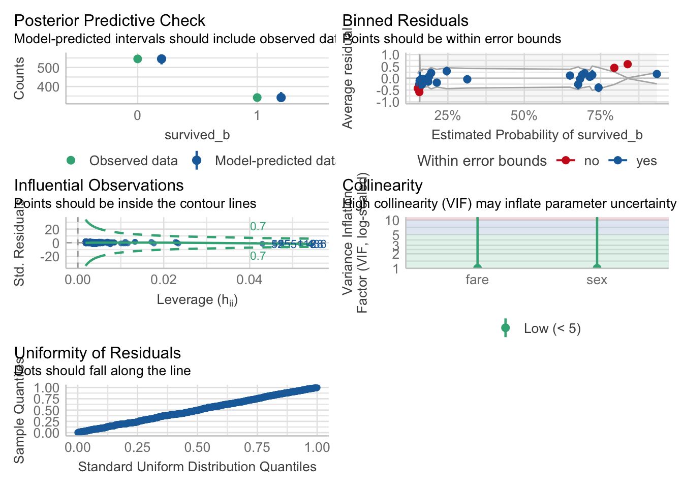
COMPARE THE PPP CHECKS BETWEEN THE MODELS?
Now, let’s take a look at the case for more complex models with one dummy coded categorical predictor variable and two continuous predictors with an interaction term.
Again, before we fit the binary regression, it would be worthwhile to try fitting the less appropriate regular general linear model. We’ll use our old friend lm() to assess the relationship between the outcome variable survived_b with the predictor variables sex, fare, and age. For more information on general linear modeling, we covered these topics in our Regression Recap chapter.
Here, we will focus our example with an interaction between sex and age.
| Parameter | Coefficient | SE | 95% CI | t(882) | p |
|---|---|---|---|---|---|
| (Intercept) | 0.58 | 0.05 | (0.48, 0.68) | 11.41 | < .001 |
| sex (male) | -0.33 | 0.06 | (-0.46, -0.21) | -5.16 | < .001 |
| fare | 1.58e-03 | 2.77e-04 | (1.04e-03, 2.12e-03) | 5.69 | < .001 |
| age | 3.24e-03 | 1.65e-03 | (1.96e-06, 6.47e-03) | 1.96 | 0.050 |
| sex (male) × age | -6.54e-03 | 2.02e-03 | (-0.01, -2.58e-03) | -3.24 | 0.001 |
As the results show, we have a significant effect of fare, such that a 1 unit increase in fare increases the chance of survival by a small amount (0.00158 units of “survival”) while controlling for sex and age. In addition, we see significant effects of our dummy coded sex variable both as the intercept difference from 0 being significant (i.e., the reference group being females with an average survival of 0.58 units), and a significant difference between males and females (i.e, a decrease of 0.33 survival units for males). There is also a significant partial effect of age while controlling fare and sex, and a significant sexxage interaction term.
Despite the challenge of interpreting what units of survival are, it is worth nothing that the regular lm() “worked” in that it was able to produce an estimate.
However, it doesn’t mean that the model is the best model to use and this is evident when we plot the predictions using the predict_response() function for fare.
predict_response(fitlm2, terms = "fare") |> plot(show_data = TRUE)Data points may overlap. Use the `jitter` argument to add some amount of
random variation to the location of data points and avoid overplotting.
Notice that although the data points are only either 0 or 1 (binary), the regression line takes intermediate values between 0 and 1, and extreme values above 1! For example, if a passenger paid $100, then the outcome value would be ~0.80, which is somewhere between alive and dead! We can’t have passengers somewhat between alive/dead, or more or less alive/dead!
When we fit a model, we always want to see if there were any violations in the assumptions. When using the general linear model via the lm() function for binary responses, taking a look at a plot of the residuals, using check_residuals() 2, should be concerning.
## Check residuals
check_residuals(fitlm2) |> plot() # looks bad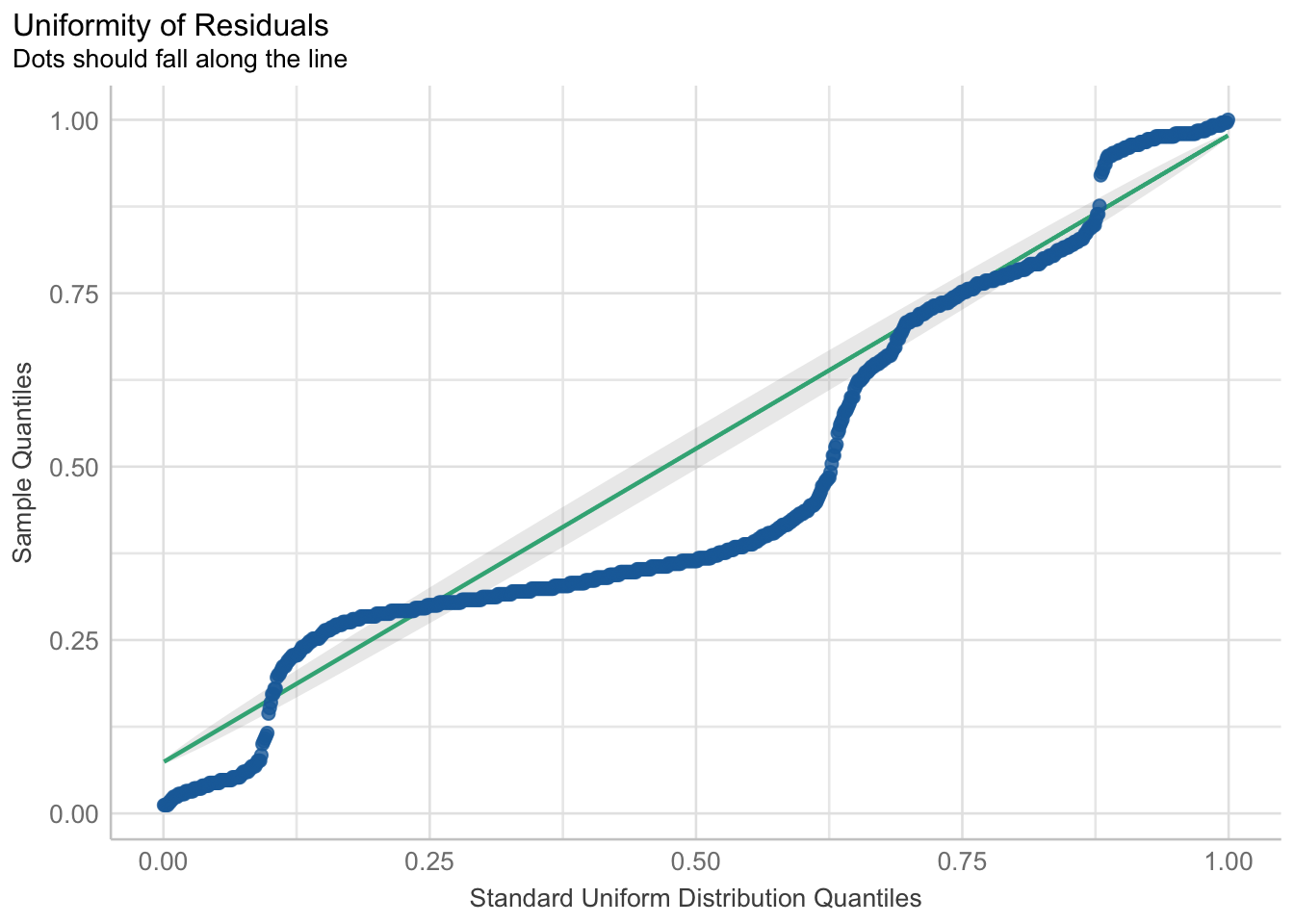
Yikes! As you can see, the dots do not fall along the line. Once this or any other assumption of the general linear model are not met, this is a clear sign that parts of the model may not be trustworthy. Specifically, in this case of the non-uniformity of residuals, there is terrible violation to the model’s uncertainty estimates; therefore, while the predictions may be okay, we can (and should) do better.
Now let’s compare our modeling of the same variables using binary/logistic regression on the interpretation of estimates and adherence to model assumptions.
“Is there a relationship between the amount of fare, sex, and the log-odds of survival?”
Again, because we have multiple predictors, multiple regression allows us to control for the effects of multiple predictors on the outcome, and we are left with the unique effect of a predictor when controlling for other predictors. In this case, the outcome variable will be survived_b, and the predictor variables will be sex (categorical variable), fare (continuous variable), and age (continuous variable).
We did a lot of work already with the lm() in the “Regression Recap”. The glm() function is in many ways the same as the lm() function. Even the syntax for how we write the equation is the same. In addition, we can use the same model_parameters() function to get our table of parameter estimates. Indeed, we will use the glm() function for the remainder of the rest of the online modules.
But notice that the glm() function has one more input argument. This input argument is the “family” input argument, which requires which “family of distributions” to use and which “link function” choice. For binary regression, we supply the binomial distribution and the logit link function.
| Parameter | Log-Odds | SE | 95% CI | z | p |
|---|---|---|---|---|---|
| (Intercept) | 0.18 | 0.29 | (-0.39, 0.75) | 0.61 | 0.544 |
| sex (male) | -1.26 | 0.38 | (-2.01, -0.52) | -3.31 | < .001 |
| fare | 0.01 | 2.35e-03 | (7.05e-03, 0.02) | 4.85 | < .001 |
| age | 0.02 | 0.01 | (-1.59e-03, 0.04) | 1.77 | 0.076 |
| sex (male) × age | -0.04 | 0.01 | (-0.07, -0.02) | -3.23 | 0.001 |
Again, the parameter table output from a model fit with glm() looks very similar to parameter table outputs from models fit with lm(). But there is a big difference – in glm() models, we are no longer working in the same raw units!
This difference is apparent in the second column of the output table: “Log-Odds”. Because we fit a logistic regression with a logit function, the parameter values are in “log-odds” unit.
Due to the nature of the dummy coded categorical variable sex, we will assess the parameters from each level of that variable first.
The intercept is the average log-odds of surviving for female passengers while accounting for the simple effects of
fareandage. In this case, female passengers at 0 years old and no fare have an average log odds of 0.18 indiciating that female passengers are more likely to survive than not survive.
Male passengers have a 1.26 decrease in the log-odds of suriving relative to the female passengers while accounting for the simple effects of
fare(at $0) andageat 0 years old (i.e., they have a worse chance of surviving).
Because the intercept was not significant, there was no significant difference between the estimate of female passengers and 0. Because “sex[male]” was significant, the difference between female and male passengers was significant, \(p<0.001\).
While controlling for the simple effects of
sex(for females) andage(at 0 years old), a one unit increase infarewas significantly related to a 0.01 increase in the log-odds of survival.
While controlling for the simple effects of
sex(for females) andfare(at $0), a one unit increase inagewas significantly related to a 0.02 increase in the log-odds of survival.
We now turn our attention to the continuous variable fare and age. Both estimates are positive (greater than 0), so it is the case that we can say it is more likely for someone to survive the Titanic with an increase in fare paid and age.
This simple effect (fare) is also statistically significant from 0 (\(p<0.001\)).
This simple effect (age) is not statistically significant from 0 (\(p=0.08\)).
The
sexxageinteraction term was statistically significant (\(p<0.001\)). So, the slope of age will decrease in log odds by 0.04 for male passengers, and the male-female difference will decrease in log odds by 0.04 for every unit increase in age.
We can easily convert log-odds to odds. In order to convert from a log-odds to odds, we just need to take the exponentiate the parameter value.
Fortunately, we can actually transform the entire log-odds parameter table results into odds using the same model_parameters() function with the added input argument of “exponentiate”, like so:
model_parameters(fit2, exponentiate = TRUE) |> print_md()| Parameter | Odds Ratio | SE | 95% CI | z | p |
|---|---|---|---|---|---|
| (Intercept) | 1.19 | 0.35 | (0.68, 2.11) | 0.61 | 0.544 |
| sex (male) | 0.28 | 0.11 | (0.13, 0.60) | -3.31 | < .001 |
| fare | 1.01 | 2.38e-03 | (1.01, 1.02) | 4.85 | < .001 |
| age | 1.02 | 0.01 | (1.00, 1.04) | 1.77 | 0.076 |
| sex (male) × age | 0.96 | 0.01 | (0.94, 0.98) | -3.23 | 0.001 |
The intercept is the average odds ratio of surviving for female passengers while accounting for the simple effects of
fareandage. In this case, female passengers at 0 years old and no fare have an average odds of 1.19 indiciating that female passengers are more likely to survive than not survive.
Male passengers have a 0.72 decrease, or 72% decrease, in the odds of suriving relative to the female passengers while accounting for the simple effects of
fareandage(i.e., they have a worse chance of surviving). It is a decrease because we are talking in odds and the value is less than 1. And we interpret that value as 0.72 because 1 - 0.28 = 0.72.
Because the intercept was not significant, there was no significant difference between the estimate of female passengers and 0. Because “sex[male]” was significant, the difference in odds between female and male passengers was significant, \(p<0.001\).
While controlling for the simple effects of
sexandage, a one unit increase infarewas significantly related to a 0.01 increase, or 1% increase, in the odds of survival. It is an increase because we are talking in odds and the value is greater than 1. And we interpret that value as 0.01 because 1.01 - 1 = 0.01.
While controlling for the simple effects of
sexandfare, a one unit increase inagewas significantly related to a 0.02 increase, or 2% increase, in the odds of survival. It is an increase because we are talking in odds and the value is greater than 1. And we interpret that value as 0.02 because 1.02 - 1 = 0.02.
We now turn our attention to the continuous variable fare and age. Both estimates are positive (greater than 0), so it is the case that we can say it is more likely for someone to survive the Titanic with an increase in fare paid and age.
This simple effect (fare) is also statistically significant from 0 (\(p<0.001\)).
This simple effect (age) is not statistically significant from 0 (\(p=0.08\)).
The
sexxageinteraction term was statistically significant (\(p<0.001\)). So, the slope of age will decrease in odds by 0.04, or 4% decrease, for male passengers, and the male-female difference will decrease in odds by 0.04, or 4% decrease, for every unit increase in age.
A convenient transformation is taking the log-odds and converting into probability. Then, our question becomes “Is there a relationship between the sex, fare, age, and the probability of survival?”.
For models with an interaction term, we can assess the interaction term with the ggpredict() function. It can be used to visualize the interaction term with a marginal effects, or “spotlight”, plot. Here, we can see the differing probabilities of survival for each sex by age while accounting for the effect of fare.
Data were 'prettified'. Consider using `terms="age [all]"` to get smooth
  plots.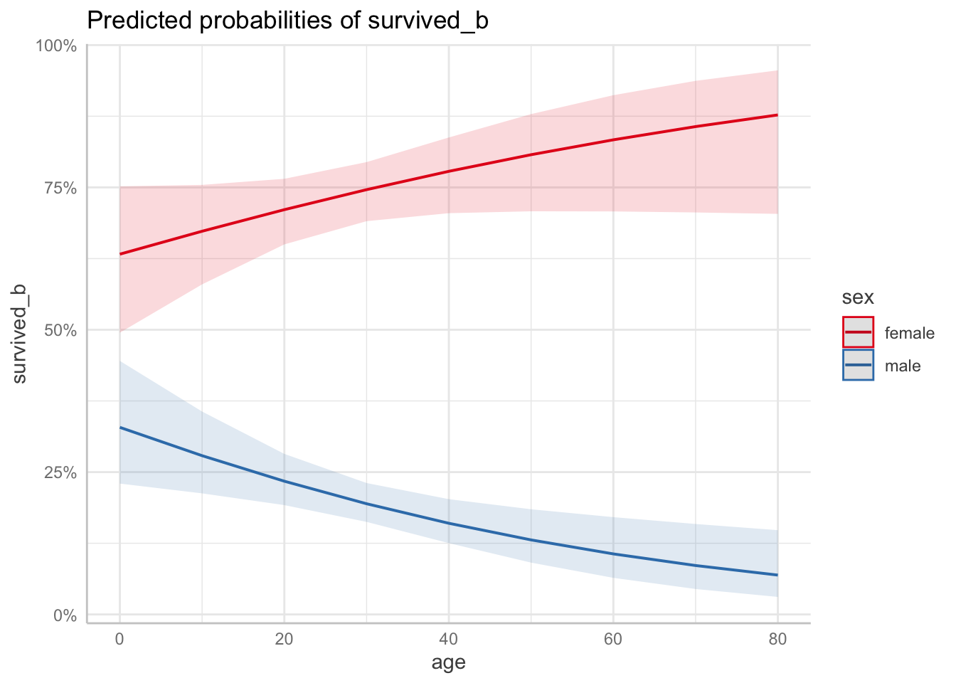
We can also assess this probabilities with the predict_response() function. It outputs a plot with the Y-axis as “the probability of survival_b” and the X-axis as the predictor (in this case fare) in raw units.
With predicted probabilities, while accounting for sex and age, we can see the probability of surviving is increasing with fare amount.
predict_response(fit2, terms = "fare") |> plot(show_data = TRUE)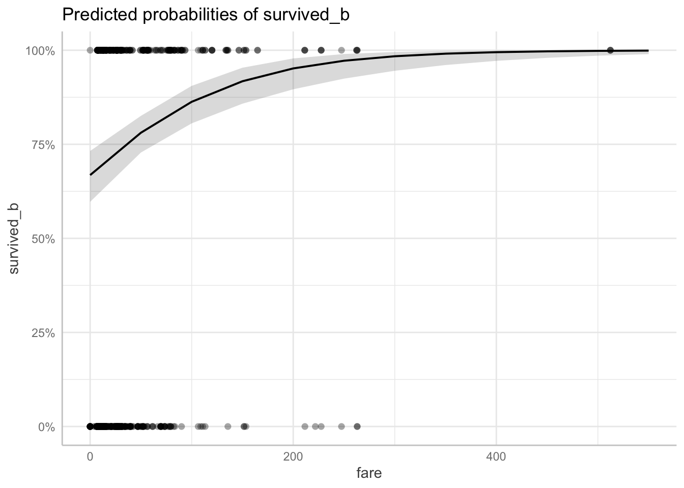
We can also plot the predicted probabilities of sex while accounting for the effect of fare and age.
predict_response(fit2, terms = "sex") |> plot(show_data = TRUE)
When the predicted probabilities are plotted, we can visualize the differences in probabilities of surviving between each sexes.
Additionally, we can see the exact probability value for each class with the estimate_means() function.
| sex | Probability | 95% CI |
|---|---|---|
| female | 0.74 | (0.69, 0.79) |
| male | 0.20 | (0.16, 0.23) |
Variable predicted: survived_b; Predictors modulated: sex; Predictors averaged: fare (32), age (29); Predictions are on the response-scale.
When we use logistic regression over regular linear regression, we benefit in terms of adhering to the assumptions of the linear model. First, let’s see if our residuals are better when we used the GLM.
As we can see, compared to our residuals plot using lm(), our glm() logistic model conforms to the uniformity of residuals assumptions way better.
## Check residuals
check_residuals(fit2) |> plot() # looks way better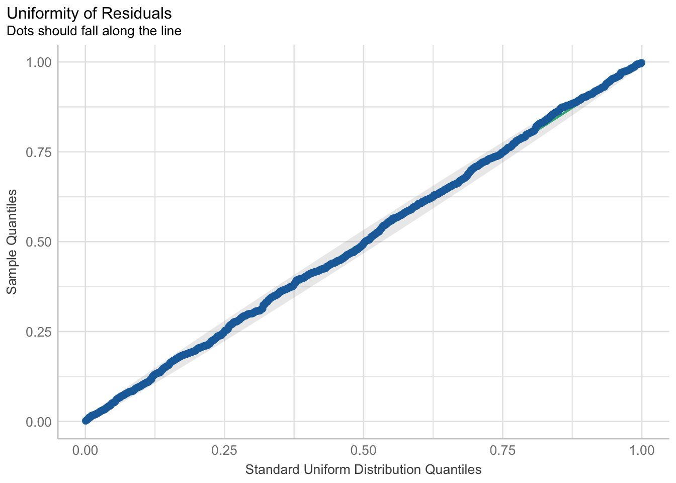
Overall, we can see the benefit of the glm() against the lm() when we compare between the two models that have the same outcome and predictors.
check_model(fitlm2)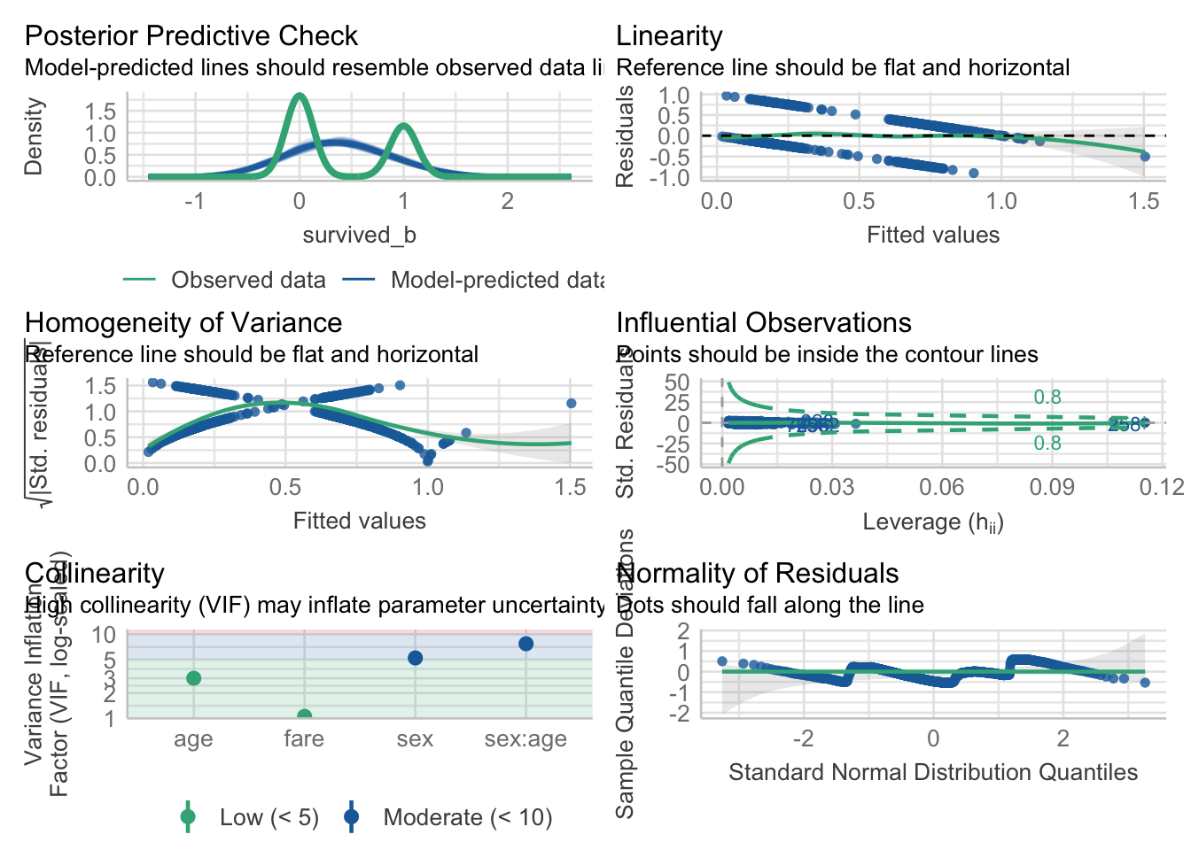
check_model(fit2)