# A tibble: 297 × 13
     sex children finances support dcl_1 dcl_2 dcl_3 dcl_4 dcl_5 dcl_6 dcl_7
   <dbl>    <dbl>    <dbl>   <dbl> <dbl> <dbl> <dbl> <dbl> <dbl> <dbl> <dbl>
 1     0        0        0   2.54      1     1     1     1     1     1     1
 2     1        1        1   3.92      1     1     1     1     1     1     1
 3     1        0        2   4         0     0     0     0     0     0     0
 4     0        0        1   1.42      1     1     1     1     0     1     0
 5     1        1        1   0.958     1     1     1     1     1     1     1
 6     0        0        2   2.92      0     0     0     0     0     0     0
 7     0        1        1   3.21      1     1     1     1     1     1     1
 8     1        1        1   2.33      0     0     0     0     0     0     0
 9     1        1        2   2.42      0     0     1     1     1     0     0
10     0        0        1   2.33      1     1     1     1     1     1     1
# ℹ 287 more rows
# ℹ 2 more variables: dcl_8 <dbl>, dcl_9 <dbl>4 Bounded Count Regression
4.1 Binomial Regression with Bounded Counts
When your outcome variable is a bounded count variable, it has a lower bound of 0 and a fixed upper bound. Specifically, each value of this variable represents the proportion of a success, or presence/endorsement, of that value; in other words, each value in that outcome variable can be thought of as a binary proportion. We can use what’s called a weighted binomial regression to model this bounded count variable.
A bounded count variable is easiest to understand and identify with an example. Imagine a test that is made up of 10 questions. To obtain a score on this test, you count how many questions were answered correct out of the 10 questions. In this case, each specific question is made up of a binary event (correct or incorrect). So, the minimum score on this test is 0, and the maximum score on this test is 10. And when we have many people take this test, we get a distribution of scores that can represent the probability/proportion correct of this outcome variable.
Therefore, when we can represent the probability/proportion correct of a fixed upper bound of an outcome variable, based on the success/failure or presence/absence of each value in that outcome variable, we can update binary regression very easily as a weighted binomial regression.
Also, in this treatment of the data, the items are interchangeable in terms of their order. So like in our example of a test that is made up of 10 questions, if the final score for one test-taker is a 5/10, we do not care which 5 questions were correct – this person’s score is treated as any 5 questions correct out of 10. This plays a role in how we interpret the model results later.
4.2 Data Demonstration
The data for this weighted binomial regression section features a bounded count variable in the form of a score on the Patient Health Questionnaire (PHQ-9). The score on this self-report questionnaire involves adding up the total number of points assigned to each of 9 questions (where each question is worth 3 points); therefore, the minimum score for any patient is 0, and the maximum score is 27 points. According to the PHQ-9, the higher the score, the more severe depression a patient has.
Notice that when talking about the score for any patient who takes this questionnaire, we are only concerned with the final score out of 27 points, and we do not make a big deal about any one question on the exam, or the order of the questions. So, we are treating the items on this questionnaire as interchangeable.
The question we will ask and answer with weighted binomial regression is what can predict a high PHQ-9 score. First, we will consider as our main predictor variable the income_ratio variable where the higher the amount of this ratio, the more income one has relative to debt.
Data: depression.csv
Data: depression_checklist.csv
4.3 Loading the Packages and Reading in Data
In addition to our usual packages (tidyverse, easystats, and ggeffects), we will also need to load DHARMa and qqplotr in order to make our plots for our weighted binary regression models.
This data shows records for 297 patients screened with the DCL-9 where each row is one participant.
Here’s a table of our variables in this dataset:
| Variable | Description | Values | Measurement |
|---|---|---|---|
sex |
Sex of Participant (0 = Female, 1 = Male) | Integer | Ordinal |
children |
Has Children (0 = no, 1 = yes) | Integer | Nominal |
finances |
Amount of Money Per Month (0 = not enough, 1 = just enough, 2 = some extra) | Integer | Ordinal |
support |
Amount of Social Support | Double | Scale |
dcl1 to dcl9
|
Depression Symptoms (0 = absent, 1 = present) | Integer | Ordinal |
4.4 Prepare Data / Exploratory Data Analysis
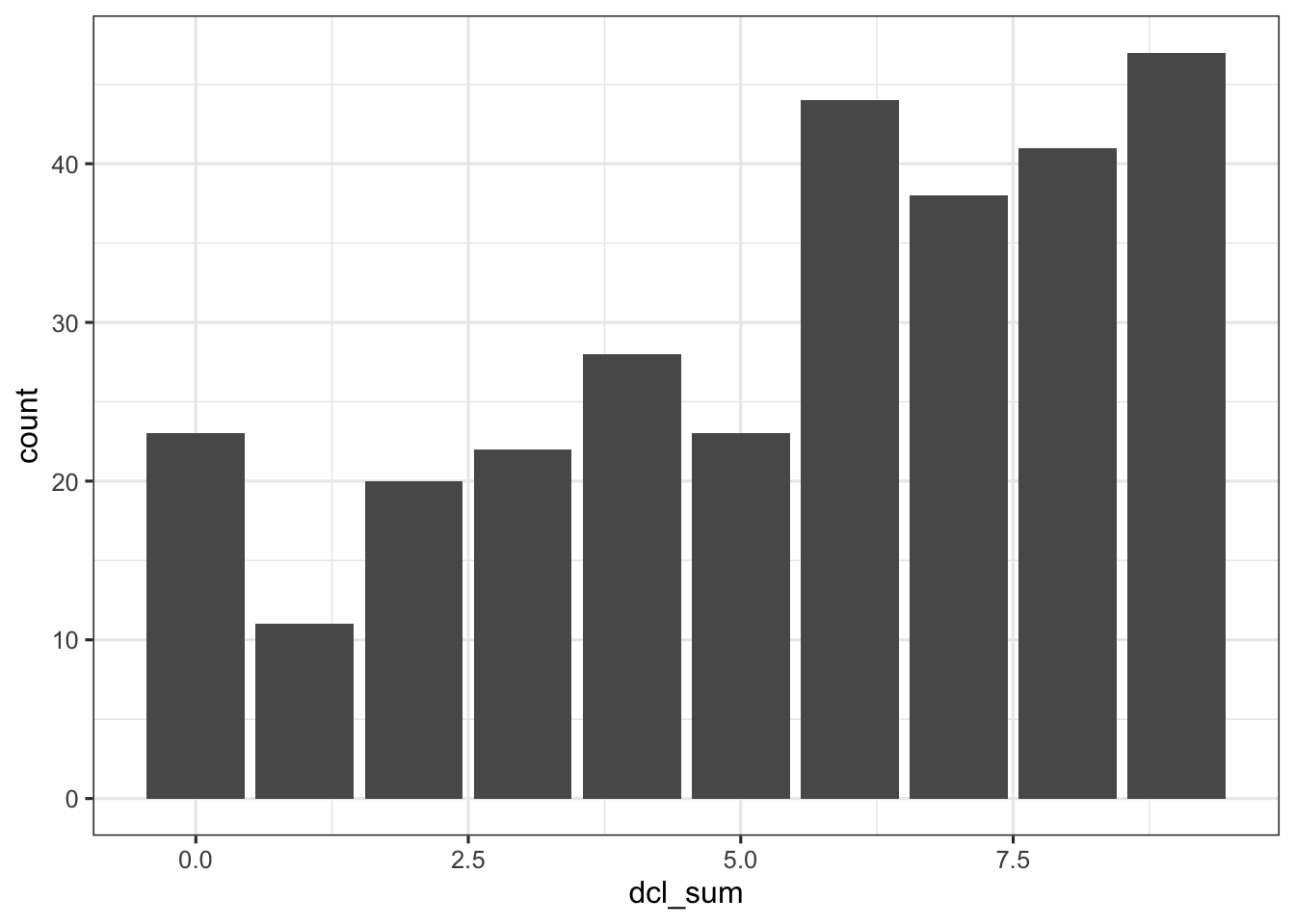
For weighted binomial regression, in order to model the DCL-9 score as the outcome variable, we need to re-code each DCL score for each participant as a weighted proportion out of the max score of 9. Here, we will use the mutate() function from the dplyr package (which is a package that automatically loaded with tidyverse) to add a three new columns to our data: the first will be dcl_max which is the max score (9) any one participant can have on the DCL-9, the second is dcl_sum which is the total sum score across all DCL-9 questions, and the third column is dcl9_p, which is hte weighted proportion, or fraction, for a participant out of max score of 9.
# depression2 <-
#   depression |>
#   mutate(
#     phq9_max = 27, # maximum possible score (can be same or different per row)
#     phq9_p = phq9 / phq9_max # proportion of maximum possible score per row
#   )

depression2 <-
  depression |>
  mutate(
    dcl_max = 9,
    dcl_sum = rowSums(pick(dcl_1:dcl_9)),
    dcl9_p = dcl_sum / dcl_max
  )

depression2
# A tibble: 297 × 16
sex children finances support dcl_1 dcl_2 dcl_3 dcl_4 dcl_5 dcl_6 dcl_7
<dbl> <dbl> <dbl> <dbl> <dbl> <dbl> <dbl> <dbl> <dbl> <dbl> <dbl>
1 0 0 0 2.54 1 1 1 1 1 1 1
2 1 1 1 3.92 1 1 1 1 1 1 1
3 1 0 2 4 0 0 0 0 0 0 0
4 0 0 1 1.42 1 1 1 1 0 1 0
5 1 1 1 0.958 1 1 1 1 1 1 1
6 0 0 2 2.92 0 0 0 0 0 0 0
7 0 1 1 3.21 1 1 1 1 1 1 1
8 1 1 1 2.33 0 0 0 0 0 0 0
9 1 1 2 2.42 0 0 1 1 1 0 0
10 0 0 1 2.33 1 1 1 1 1 1 1
# ℹ 287 more rows
# ℹ 5 more variables: dcl_8 <dbl>, dcl_9 <dbl>, dcl_max <dbl>, dcl_sum <dbl>,
# dcl9_p <dbl>In addition, we will change all the discrete variables to factors.
depression2$sex <- factor(depression2$sex, levels = c(0,1),
                          labels = c("Female","Male"))
depression2$children <- factor(depression2$children, levels = c(0,1),
                               labels = c("NoChildren","Children"))

depression2$finances <- factor(depression2$finances, levels = c(0,1,2),
                               labels= c("NotENough","Enough","SomeExtra"))
4.4.1 Dealing with Missingness
It is worth noting that in this toy data set, the max score for any participant is always going to be “9” because there is no missing data. If there is missing data, the max score for any one row may be different. We can still use weighted binomial regression with bounded counts with data with missing values if we adjust the max score for any rows with missing values.
Let’s load in the same DCL data set but with missing values in DCL scores in each row.
## Read in data from file
depression_m <- read_csv("depression_checklist_m.csv")
Rows: 297 Columns: 13
── Column specification ────────────────────────────────────────────────────────
Delimiter: ","
dbl (13): sex, children, finances, support, dcl_1, dcl_2, dcl_3, dcl_4, dcl_...
ℹ Use `spec()` to retrieve the full column specification for this data.
ℹ Specify the column types or set `show_col_types = FALSE` to quiet this message.depression_m# A tibble: 297 × 13
sex children finances support dcl_1 dcl_2 dcl_3 dcl_4 dcl_5 dcl_6 dcl_7
<dbl> <dbl> <dbl> <dbl> <dbl> <dbl> <dbl> <dbl> <dbl> <dbl> <dbl>
1 0 0 0 2.54 1 1 1 1 1 NA 1
2 1 1 1 3.92 1 1 1 1 1 1 1
3 1 0 2 4 0 0 0 0 0 0 0
4 0 0 1 1.42 1 1 1 1 0 1 0
5 1 1 1 0.958 NA 1 1 1 1 1 1
6 0 0 2 2.92 0 0 0 NA 0 0 0
7 0 1 1 3.21 1 1 1 1 1 1 1
8 1 1 1 2.33 0 0 0 0 0 0 0
9 1 1 2 2.42 0 0 1 1 1 0 NA
10 0 0 1 2.33 1 1 1 1 NA 1 1
# ℹ 287 more rows
# ℹ 2 more variables: dcl_8 <dbl>, dcl_9 <dbl>When there is missing NA values for scores in our measure, we can slightly adjust our code to reflect a different max score for each row (thus, the weight for each row is different).
# A tibble: 297 × 16
     sex children finances support dcl_1 dcl_2 dcl_3 dcl_4 dcl_5 dcl_6 dcl_7
   <dbl>    <dbl>    <dbl>   <dbl> <dbl> <dbl> <dbl> <dbl> <dbl> <dbl> <dbl>
 1     0        0        0   2.54      1     1     1     1     1    NA     1
 2     1        1        1   3.92      1     1     1     1     1     1     1
 3     1        0        2   4         0     0     0     0     0     0     0
 4     0        0        1   1.42      1     1     1     1     0     1     0
 5     1        1        1   0.958    NA     1     1     1     1     1     1
 6     0        0        2   2.92      0     0     0    NA     0     0     0
 7     0        1        1   3.21      1     1     1     1     1     1     1
 8     1        1        1   2.33      0     0     0     0     0     0     0
 9     1        1        2   2.42      0     0     1     1     1     0    NA
10     0        0        1   2.33      1     1     1     1    NA     1     1
# ℹ 287 more rows
# ℹ 5 more variables: dcl_8 <dbl>, dcl_9 <dbl>, dcl_max <dbl>, dcl_sum <dbl>,
#   dcl9_p <dbl>
4.4.2 Plotting Relationships in DCL-9
First let’s consider the shape of the distribution of the counts/scores.
Let’s first plot to see any relationship between the support and the weighted DCL-9 score (dcl9_p). We tend to see that more of the data points, especially at higher DCL-9 scores, fall in the higher values of support which suggests a positive relationship between support and depression severity; in other words, the higher the support, the higher the score on the DCL-9 (and more depression symptoms). While this may seem visually counter-intuitive, note that it is possible that most people in our sample may have depression symptoms despite having support, and that the plot is misleading (especially since the amount of dcl9_p scores are visually about the same across the higher levels of support).
ggplot(depression2, aes(x = support, y = dcl9_p)) +
  geom_point() + mytheme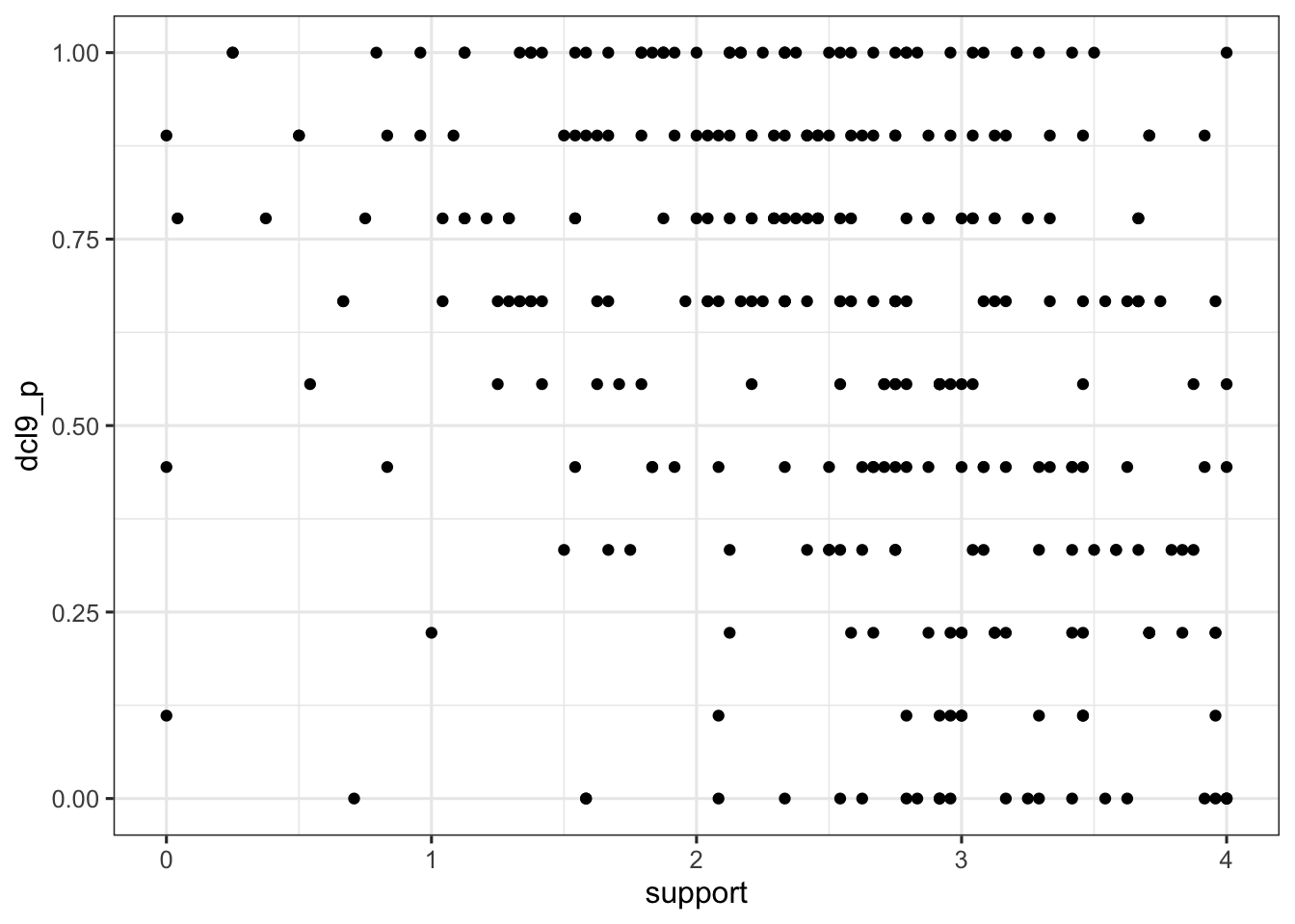
5 Models Without Interaction Terms
First, let’s take a look at the case for models with one dummy coded categorical predictor variable and one continuous predictor without any interaction term.
5.1 Less Correct: the General Linear Model
Before we fit the binary regression, it would be worthwhile to try fitting the less appropriate regular general linear model. We’ll use our old friend lm() to assess the relationship between the outcome variable dcl9_p with the predictor variables support and sex. For more information on general linear modeling, we covered these topics in our Regression Recap chapter.
6 Fitting the Weighted Binomial Regression Models
6.1 One Continous Predictor
When we fit our weighted binomial regression, we now will use the glm() function.
We did a lot of work already with the lm() in the “Regression Recap”. The glm() function is in many ways the same as the lm() function. Even the syntax for how we write the equation is the same. In addition, we can use the same model_parameters() function to get our table of parameter estimates. Indeed, we will use the glm() function for the remainder of the rest of the online modules.
But for weighted binomial regression, notice that the glm() function has two more input arguments. These input arguments are the “family” input argument, which requires which “family of distributions” to use and which “link function” choice, and a “weights” argument, which is a column in the dataset that represents the max score for each proportion.
For weighted binary regression, we supply the binomial distribution and the logit link function into the “family” input argument, and dcl9_max column name for the “weights” input argument.
As mentioned before, we will consider the effect of support.
We then assess the results with model_paramters().
# fit1 <- glm(
#   formula = dcl9_p ~ sex + support,
#   family = binomial(link = "logit"),
#   weights = dcl_max,
#   data = depression2
# )
#
# model_parameters(fit1) |> print_md()
# fit1 <- glmmTMB(
# formula = dcl9_p ~ sex + support,
# family = betabinomial(link = "logit"),
# weights = dcl_max,
# data = depression2
# )6.1.1 Parameter Table Interpretation (Log-odds)
Again, the parameter table output from a model fit with glm() looks very similar to parameter table outputs from models fit with lm(). But there is a big difference – in glm() models, we are no longer working in the same raw units!
This difference is clear in the second column of the output table: “Log-Odds”. Because we fit a logistic regression with a logit function, the parameter values are in “log-odds” unit. Technically, when support is in log-odds units, we can only say:
For every one 1 unit increase in
support, there is a 0.52 decrease in the log-odds of having a one-unit higher DCL-9 score.
Although this is technically true, it isn’t at first clear what it means to have a “0.52 unit decrease in log-odds of dcl9_p”. Let’s interpret the \(-0.52\) log-odds value:
If log-odds $ = -0.52$, then it is less than 0, meaning it is more likely to have a lower DCL-9 score (than a higher DCL-9 score) when we use
supportas a predictor.This effect is also statistically significant from 0 (\(p<0.001\)). Remember, with log-odds, a value of 0 means it is equally likely for an event to occur or not occur. In this case, since it is significantly less than 0, we can say it is more likely to not have a symptom than have a symptom (i.e. score less on the DCL-9 than score more) when predicted by
support.As mentioned before, with weighted binomial regression the values of the outcome variable are interchangeable, so our parameter results speak in reference to obtaining one value difference on the outcome variable. In other words, we are estimating the likelihood of endorsing any single symptom of depression. Therefore, when log-odds \(= -0.52\), that is in reference to decreasing (because it is negative) the outcome variable score by one value lower.
6.1.2 Parameter Table Interpretation (Odds)
We can also present the results in odds ratios by using the “exponentiate” input argument.
#model_parameters(fit2, exponentiate = TRUE) |> print_md()Now that we are in odds, we can adjust our previous interpretation of the support parameter for odds:
For every one unit increase in
support, there is a 0.40 decrease, or a 40% decrease, in the odds of having a one-unit higher DCL-9 score.
Recall that when odds \(=1\), that means both events are equally likely to happen. So for example, here we read an odds value of \(0.60\), then we only consider the differences from 1 as meaningful. In this case, that is a decrease of 0.40, or 40%, from our baseline value of 1.
Also from the output table, we know the significance values in odds and we can now say that the effect of support in the decrease of odds is statistically significant from 1, \(p<0.001\) 1
A lot of fields, like medicine, prefer to output and report their logistic regression values in odds.
6.1.3 Predicted Probability
A convenient transformation is taking the log-odds and converting into probability. Then, our question becomes “Is there a relationship between support and the probability of scoring one value different on the DCL-9?”.
We can assess this relationship with the predict_response() function. It outputs a plot with the Y-axis as “the probability of DCL-9” and the X-axis as the predictor (in this case support) in raw units, and it overlays the predicted probability on top of the data.
#predict_response(fit2, terms = "support") |> plot(show_data = TRUE)Again, the transformed outcome variable is the “probability of dcl9_p” (on the y-axis), so we can see that it is bounded between [0,100]. The logistic regression line also makes predictions between these bounds so we no longer have the model predicting unreasonable values/states which would happen if we didn’t consider using the glm() function. Lastly, we can now see how an increase in suppport leads to a decrease in the probability of scoring one score lower on the DCL-9.
Also notice that our prediction line is more in agreement with the general intuition that the higher support one has, the less depression symptoms one may have. This is more clear now that the model can pick apart this relationship that would be hard to see if we only relied on a solely visual inspection.
TipWhy not always use probability?
Although working with probabilities seems to be more easily understandable, we cannot have parameter estimates in probabilities. Therefore, results are often communicated in logits or odds since we can have estimates, uncertainty values (like standard deviations), and significance tests applied to them.
## Two Continous Predictors
“Is there a relationship between the support, age, and the score on the PHQ-9?”
When we have two predictors, we are now conducting a multiple weighted binomial (logistic) regression. Recall that multiple regression, in general, allows us to control for the effects of multiple predictors on the outcome, and we are left with the unique effect of a predictor when controlling for other predictors.
Once again, let’s fit this model with the glm() function.
# fit3 <- glm(
#   formula = phq9_p ~ income_ratio + age,
#   family = binomial(link = "logit"),
#   weights = phq9_max,
#   data = depression2
# )
#
# ## Print parameters in logit (i.e., log-odds) units
# model_parameters(fit3) |> print_md()
6.1.4 Parameter Table Interpretation (Log-odds)
When the parameter table is in log-odds, we can now say the following:
For every one unit increase in
income_ratio, there is a 0.16 decrease in the log-odds of having a one-unit higher PHQ-9 score (and greater chance of having severe depression) while controlling for the effect ofage. The unique (i.e., partial) effect ofincome_ratiois significantly different from 0, \(p<0.001\).
For every one unit increase in
age, there is a 6.95e^-3 increase (because it is positive) in the log-odds of having a one-unit higher PHQ-9 score (and a greater chacne of having severe depression) when controlling for the effect ofincome_ratio. The unique (i.e., partial) effect ofageis significantly different from 0, \(p<0.01\).
Remember, in log-odds, if the value is positive, it is more likely for the event to occur, and if it is negative, it is more likely for the event to not occur.
6.1.5 Parameter Table Interpretation (Odds)
We can also present the results in odds.
## Print parameters in odds
# model_parameters(fit3, exponentiate = TRUE) |> print_md()
When the parameter table is in odds, we can now say the following:
For every one unit increase in
income_ratio, there is a 0.15 decrease, or 15.0% decrease, in the odds ratio of having a one-unit higher PHQ-9 score when controlling for the effect ofage. The unique (i.e., partial) effect offareis significantly different from 0, \(p<0.01\).
For every one unit increase in
age, there is a 0.01 increase, or 1.0% increase, in the odds ratio of having a one-unit higher PHQ-9 score when controlling for the effect ofincome_ratio. The unique (i.e., partial) effect ofageis significantly different from 0, \(p<0.001\).
Remember, in odds, if the value greater than 1, it is more likely for the event to occur, and if it less than 1, it is more likely for the event to not occur.
At this point, it is interesting to consider that the higher the income_ratio amount, then the lower the chance of a one-unit increase of scores on the PHQ-9, whereas the higher the age, then the higher the chance of a one-unit increase on the PHQ-9
6.1.6 Predicted Probability
# predict_response(fit3, terms = "income_ratio") |> plot(show_data = TRUE)
# predict_response(fit3, terms = "age") |> plot(show_data = TRUE)
The plots for predicted probabilities is helpful for highlighting the different effects for income_ratio and age on the probability of obtaining a one-unit higher score on the PHQ-9. As we see, there is a decrease in the probability of a higher score as income_ratio increases, and there is an increase in the probability of surviving as age increases.
6.2 One Dummy Coded Predictor
Let’s consider the question “Is there a relationship between gender and the log-odds/probability of scoring one-unit higher on the DCL-9?”
Remember, first we have to change our predictor variable to a factor (i.e., a dummy-coded variable), and then we can fit with glm().
# depression2$gender <- factor(depression2$gender, levels = c(0,1), labels = c("Female","Male")) #change to factor
#
# fit4 <- glm(
#   formula = dcl9_p ~ gender,
#   family = binomial(link = "logit"),
#   weights = dcl_max,
#   data = depression2
# )
#
# model_parameters(fit4) |> print_md()
6.2.1 Parameter Table Interpretation (Log-odds)
Remember, although we are performing a weighted binomial (logistic) regression, it is still dummy-coded so our parameters estimates are given relative to the first category of the predictor variable. In this case, the females are the reference group.
The intercept is the average log-odds of scoring one unit higher on the DCL-9 for females. In this case, females have a 0.29 log-odds of scoring one unit higher on the DCL-9, which means it is more likely for them to score one unit higher on the DCL-9 (since it is a log odds greater than 0)
Men have a 0.24 increase in the log-odds of scoring one unit higher on the PHQ-9 relative to women (i.e., they have greater chance of scoring higher).
There was a significant difference in the log-odds women from 0, \(p<0.001\). The difference between women and men was significant, \(p<0.01\).
6.2.2 Estimating means and plots
# gmeans1 <- estimate_means(fit4, by = c("gender"))
# gmeans1 |> print_md()
6.2.3 Parameter Table Interpretation (Odds)
Like in other logistic regression models, we can convert to odds ratios with model_parameters and “exponentiate” input argument.
# model_parameters(fit4, exponentiate = TRUE) |> print_md()The intercept is the average odds of scoring one-unit higher on the PHQ-9 for women. In this case, women have a base odds of 1.32 for scoring higher on the DCL-9. Since it is greater than 1, it is more likely for someone to score one-unit higher.
Men have a 0.27 increase, or 27% increase, in the odds of scoring one-unit higher on the PHQ-9 relative to women (i.e., they have a greater chance at scoring higher on DCL-9). This is because 1.27 - 1 = 0.27.
There was a significant difference for women in the odds ratio from 1, \(p<0.001\). The difference between women and men was also significant, \(p<0.01\).
In other words, both log-odds and odds ratio show that men have a increased chance of scoring one-unit higher on the DCL-9 relative to women meaning they are more likely to score for more depression symptoms than women.
6.2.4 Predicted Probability
# predict_response(fit4, terms = "gender") |> plot(show_data = TRUE)When the predicted probabilities are plotted, we can visualize the differences in probabilities of women versus men.
6.3 One Dummy Coded Predictor and One Continous Predictor
“Is there a relationship between the income ratio, gender, and the log-odds/probability of scoring one-unit higher on the PHQ-9?”
Again, multiple regression allows us to control for the effects of multiple predictors on the outcome, and we are left with the unique effect of a predictor when controlling for other predictors. In this case, the outcome variable will be phq9_p, and the predictor variables will be gender (categorical variable) and income_ratio (continuous variable).
# fit5 <- glm(
#   formula = phq9_p ~ gender + income_ratio,
#   family = binomial(link = "logit"),
#   weights = phq9_max,
#   data = depression2
# )
#
# model_parameters(fit5) |> print_md()
6.3.1 Paramter Table Interpretation (Log-odds)
The intercept is the average log-odds of scoring higher on the PHQ-9 for women, while accounting for the effect of
income_ratio. In this case, women have a average log odds of -1.44 indiciating that they are less likely to score higher on the PHQ-9 (since it is a log odds less than 0).
Men have a 0.54 decrease in the log-odds of suriving relative to women while accounting for the effect of
income_ratio(i.e., they have a worse chance of scoring higher so they have less chance of being severely depressed).
Because the intercept was significant, there was a significant difference between for women in the log odds versus 0, \(p<0.001\). In addition, the difference in log-odds between men and women was significant, \(p<0.001\).
Lastly, while controlling for the effect of
gender, a one unit increase inincome_ratiowas significantly related to a 0.14 decrease in the log-odds of scoring one-unit higher on the PHQ-9.
6.3.2 Parameter Table Interpretation (Odds Ratio)
We can also consider the results in odds ratio by using the “exponentiate” argument in model_paramters().
#model_parameters(fit5, exponentiate = TRUE) |> print_md()The intercept is the average odds of scoring higher on the PHQ-9 for women, while accounting for the effect of
income_ratio. In this case, women have a average odds of 0.24 indiciating that they are less likely to score higher on the PHQ-9 (since it is a log odds ratio than 1).
Men have a 0.40 (because 1 - 0.60 = 0.40) decrease in the odds of suriving relative to women while accounting for the effect of
income_ratio(i.e., they have a worse chance of scoring higher so they have less chance of being severely depressed).
Because the intercept was significant, there was a significant difference between for women in the odds versus 1, \(p<0.001\). In addition, the difference in odds ratio between men and women was significant, \(p<0.001\).
Lastly, while controlling for the effect of
gender, a one unit increase inincome_ratiowas significantly related to a 0.13 decrease in the odds of scoring one-unit higher on the PHQ-9.
When the parameter table is in odds, the significance test is applied to see differences from an odds value of 1. This is because, again, an odds value of 1 means that an event occurring versus not occurring is equally likely.↩︎